Functionality of fuzzyclara package (interactive)
Maximilian Weigert, Asmik Nalmpatian, Jana Gauss, Alexander Bauer
05.June 2025
vignette_shiny.RmdThis document gives an overview of the functionality provided by the
R package fuzzyclara.
Clustering
Hard clustering
cc_hard <- fuzzyclara(data        = USArrests,
                       clusters    = 3,
                       metric      = "euclidean",
                       samples     = 1,
                       sample_size = NULL,
                       type        = "hard",
                       seed        = 3526,
                       verbose     = 0)
cc_hard
## Clustering results
##
## Medoids
## [1] "New Mexico" "Oklahoma" "New Hampshire"
##
## Clustering
## [1] 2 2 2 3 2 2 3 3 2 2 3 1 2 3 1 3 3 2 1 2 3 2 1 2 3 3 3 2 1 3 2 2 2 1 3 3 3 3
## [39] 3 2 1 2 2 3 1 3 3 1 1 3
##
## Minimum average distance
## [1] 1.180717Fuzzy clustering
cc_fuzzy <- fuzzyclara(data        = USArrests,
                       clusters    = 3,
                       metric      = "euclidean",
                       samples     = 1,
                       sample_size = NULL,
                       type        = "fuzzy",
                       m           = 2,
                       seed        = 3526,
                       verbose     = 0)
cc_fuzzy
## Clustering results
##
## Medoids
## [1] "Oklahoma" "Arizona" "Tennessee"
##
## Clustering
## [1] 3 3 1 2 1 1 2 2 1 3 2 2 1 2 2 2 2 3 2 1 2 1 2 3 2 2 2 1 2 2 1 1 3 2 2 2 2 2
## [39] 2 3 2 3 3 2 2 2 2 2 2 2
##
## Minimum average weighted distance
## [1] 1.94242
##
## Membership scores
## Cluster1 Cluster2 Cluster3
## Alabama 0.2040878 0.2391714 0.5567409
## Alaska 0.3373655 0.2726496 0.3899849
## Arizona 1.0000000 0.0000000 0.0000000
## Arkansas 0.2075892 0.3966215 0.3957893
## California 0.5401685 0.2248051 0.2350264
## Colorado 0.4475538 0.2744007 0.2780455
## Connecticut 0.2348136 0.5280016 0.2371848
## Delaware 0.2906227 0.4701428 0.2392345
## Florida 0.4443412 0.2316682 0.3239905
## Georgia 0.2091524 0.2149396 0.5759081
## Hawaii 0.2482766 0.4883161 0.2634073
## Idaho 0.2209589 0.5129169 0.2661242
## Illinois 0.4666698 0.2739684 0.2593617
## Indiana 0.1344369 0.6694262 0.1961369
## Iowa 0.2311216 0.4905457 0.2783327
## Kansas 0.1310680 0.6999444 0.1689876
## Kentucky 0.1917648 0.4401893 0.3680459
## Louisiana 0.2560625 0.2412981 0.5026393
## Maine 0.2396947 0.4695769 0.2907285
## Maryland 0.4281216 0.2306369 0.3412416
## Massachusetts 0.2682437 0.5043343 0.2274220
## Michigan 0.4467571 0.2192029 0.3340400
## Minnesota 0.2158369 0.5379562 0.2462069
## Mississippi 0.2484292 0.2817416 0.4698292
## Missouri 0.2669546 0.3898602 0.3431852
## Montana 0.1922866 0.5233027 0.2844107
## Nebraska 0.1814854 0.5935543 0.2249603
## Nevada 0.4372644 0.2469118 0.3158237
## New Hampshire 0.2351771 0.4821286 0.2826942
## New Jersey 0.3025875 0.4474846 0.2499279
## New Mexico 0.4736616 0.2098122 0.3165261
## New York 0.4959333 0.2489337 0.2551329
## North Carolina 0.2984813 0.2995500 0.4019686
## North Dakota 0.2525175 0.4409055 0.3065770
## Ohio 0.1722044 0.6264071 0.2013885
## Oklahoma 0.0000000 1.0000000 0.0000000
## Oregon 0.2597840 0.4842455 0.2559705
## Pennsylvania 0.1733916 0.6187011 0.2079073
## Rhode Island 0.2938264 0.4548769 0.2512968
## South Carolina 0.2521289 0.2569116 0.4909595
## South Dakota 0.2294820 0.4627901 0.3077278
## Tennessee 0.0000000 0.0000000 1.0000000
## Texas 0.3315450 0.2977964 0.3706587
## Utah 0.2550652 0.5204090 0.2245258
## Vermont 0.2537642 0.4173744 0.3288614
## Virginia 0.1470128 0.6016305 0.2513568
## Washington 0.2420740 0.5403595 0.2175666
## West Virginia 0.2356115 0.4301945 0.3341939
## Wisconsin 0.2298126 0.5057011 0.2644864
## Wyoming 0.1652925 0.6041126 0.2305949Clustering with self-defined distance function and other distance functions
dist_function <- function(x, y) {
  sqrt(sum((x - y)^2))
}

cc_dist <- fuzzyclara(data        = USArrests,
                      clusters    = 3,
                      metric      = dist_function,
                      samples     = 1,
                      sample_size = NULL,
                      type        = "fuzzy",
                      m           = 2,
                      seed        = 3526,
                      verbose     = 0)
cc_dist
## Clustering results
##
## Medoids
## [1] "Oklahoma" "Arizona" "Tennessee"
##
## Clustering
## [1] 3 3 1 2 1 1 2 2 1 3 2 2 1 2 2 2 2 3 2 1 2 1 2 3 2 2 2 1 2 2 1 1 3 2 2 2 2 2
## [39] 2 3 2 3 3 2 2 2 2 2 2 2
##
## Minimum average weighted distance
## [1] 1.94242
##
## Membership scores
## Cluster1 Cluster2 Cluster3
## Alabama 0.2040878 0.2391714 0.5567409
## Alaska 0.3373655 0.2726496 0.3899849
## Arizona 1.0000000 0.0000000 0.0000000
## Arkansas 0.2075892 0.3966215 0.3957893
## California 0.5401685 0.2248051 0.2350264
## Colorado 0.4475538 0.2744007 0.2780455
## Connecticut 0.2348136 0.5280016 0.2371848
## Delaware 0.2906227 0.4701428 0.2392345
## Florida 0.4443412 0.2316682 0.3239905
## Georgia 0.2091524 0.2149396 0.5759081
## Hawaii 0.2482766 0.4883161 0.2634073
## Idaho 0.2209589 0.5129169 0.2661242
## Illinois 0.4666698 0.2739684 0.2593617
## Indiana 0.1344369 0.6694262 0.1961369
## Iowa 0.2311216 0.4905457 0.2783327
## Kansas 0.1310680 0.6999444 0.1689876
## Kentucky 0.1917648 0.4401893 0.3680459
## Louisiana 0.2560625 0.2412981 0.5026393
## Maine 0.2396947 0.4695769 0.2907285
## Maryland 0.4281216 0.2306369 0.3412416
## Massachusetts 0.2682437 0.5043343 0.2274220
## Michigan 0.4467571 0.2192029 0.3340400
## Minnesota 0.2158369 0.5379562 0.2462069
## Mississippi 0.2484292 0.2817416 0.4698292
## Missouri 0.2669546 0.3898602 0.3431852
## Montana 0.1922866 0.5233027 0.2844107
## Nebraska 0.1814854 0.5935543 0.2249603
## Nevada 0.4372644 0.2469118 0.3158237
## New Hampshire 0.2351771 0.4821286 0.2826942
## New Jersey 0.3025875 0.4474846 0.2499279
## New Mexico 0.4736616 0.2098122 0.3165261
## New York 0.4959333 0.2489337 0.2551329
## North Carolina 0.2984813 0.2995500 0.4019686
## North Dakota 0.2525175 0.4409055 0.3065770
## Ohio 0.1722044 0.6264071 0.2013885
## Oklahoma 0.0000000 1.0000000 0.0000000
## Oregon 0.2597840 0.4842455 0.2559705
## Pennsylvania 0.1733916 0.6187011 0.2079073
## Rhode Island 0.2938264 0.4548769 0.2512968
## South Carolina 0.2521289 0.2569116 0.4909595
## South Dakota 0.2294820 0.4627901 0.3077278
## Tennessee 0.0000000 0.0000000 1.0000000
## Texas 0.3315450 0.2977964 0.3706587
## Utah 0.2550652 0.5204090 0.2245258
## Vermont 0.2537642 0.4173744 0.3288614
## Virginia 0.1470128 0.6016305 0.2513568
## Washington 0.2420740 0.5403595 0.2175666
## West Virginia 0.2356115 0.4301945 0.3341939
## Wisconsin 0.2298126 0.5057011 0.2644864
## Wyoming 0.1652925 0.6041126 0.2305949You can also use other distance functions from the proxy package like Gower, Manhattan etc. In order to specify arguments of the distance metric (e. g. p for Minkowski distance), you can use a self-defined distance function.
cc_manh <- fuzzyclara(data        = USArrests,
                       clusters    = 3,
                       metric      = "manhattan",
                       samples     = 1,
                       sample_size = NULL,
                       type        = "hard",
                       seed        = 3526,
                       verbose     = 0)
cc_manh
## Clustering results
##
## Medoids
## [1] "New Mexico" "Oklahoma" "New Hampshire"
##
## Clustering
## [1] 2 2 2 3 2 2 1 3 2 2 3 1 2 3 1 3 3 2 1 2 3 2 1 2 3 3 3 2 1 3 2 2 2 1 3 3 3 3
## [39] 3 2 1 2 2 3 1 3 3 1 1 3
##
## Minimum average distance
## [1] 2.011671
dist_mink <- function(x, y) {
  proxy::dist(list(x, y), method = "minkowski", p = 1)
}
cc_mink <- fuzzyclara(data        = USArrests,
                       clusters    = 3,
                       metric      = dist_mink,
                       samples     = 1,
                       sample_size = NULL,
                       type        = "hard",
                       seed        = 3526,
                       verbose     = 0)
cc_mink
## Clustering results
##
## Medoids
## [1] "New Mexico" "Oklahoma" "New Hampshire"
##
## Clustering
## [1] 2 2 2 3 2 2 1 3 2 2 3 1 2 3 1 3 3 2 1 2 3 2 1 2 3 3 3 2 1 3 2 2 2 1 3 3 3 3
## [39] 3 2 1 2 2 3 1 3 3 1 1 3
##
## Minimum average distance
## [1] 2.011671Select optimal number of clusters
cc_number <- evaluate_cluster_numbers(
                       data            = USArrests,
                       clusters_range  = 2:6,
                       metric          = "euclidean",
                       samples         = 1,
                       sample_size     = NULL,
                       type            = "hard",
                       seed            = 3526,
                       verbose         = 0)
cc_number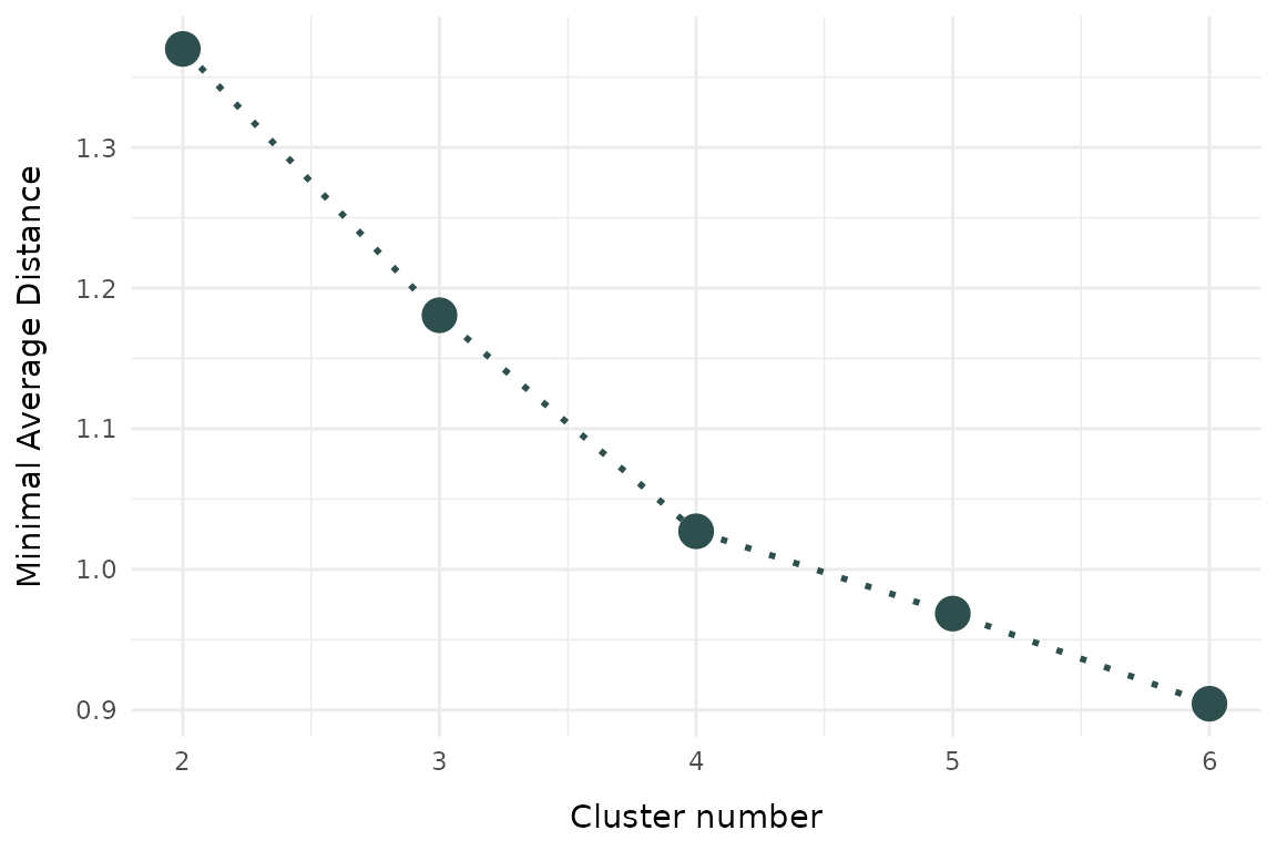
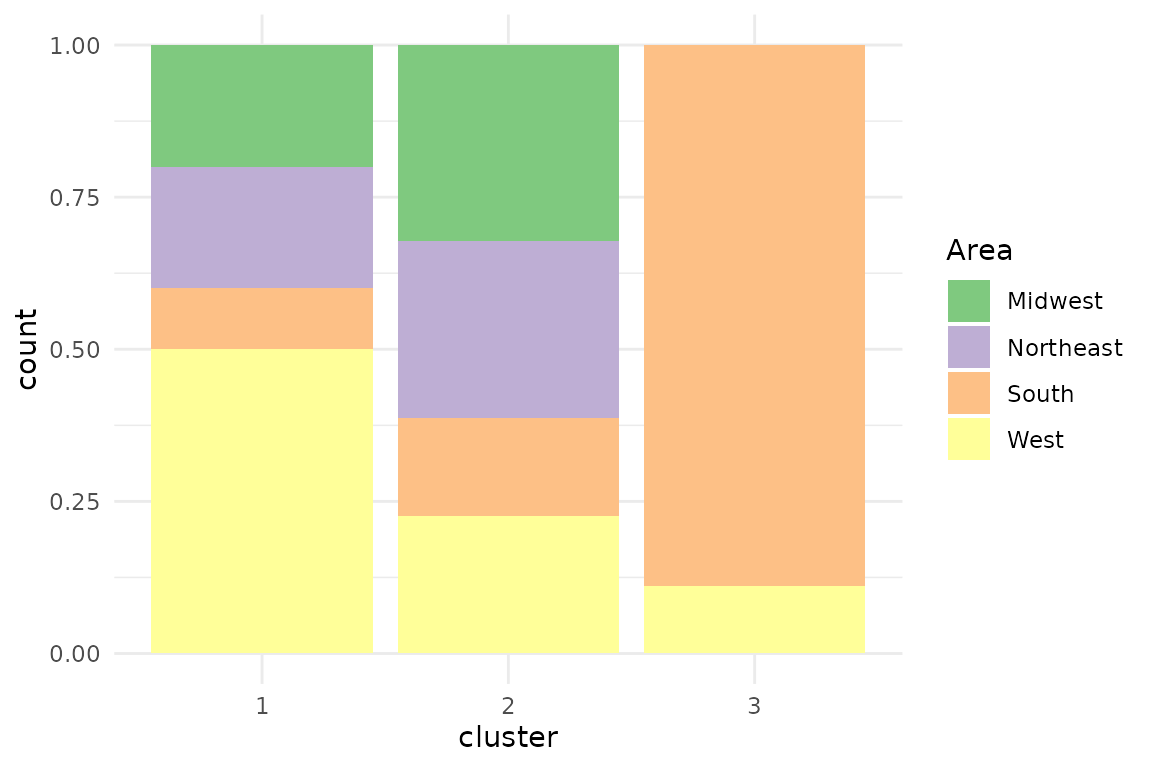
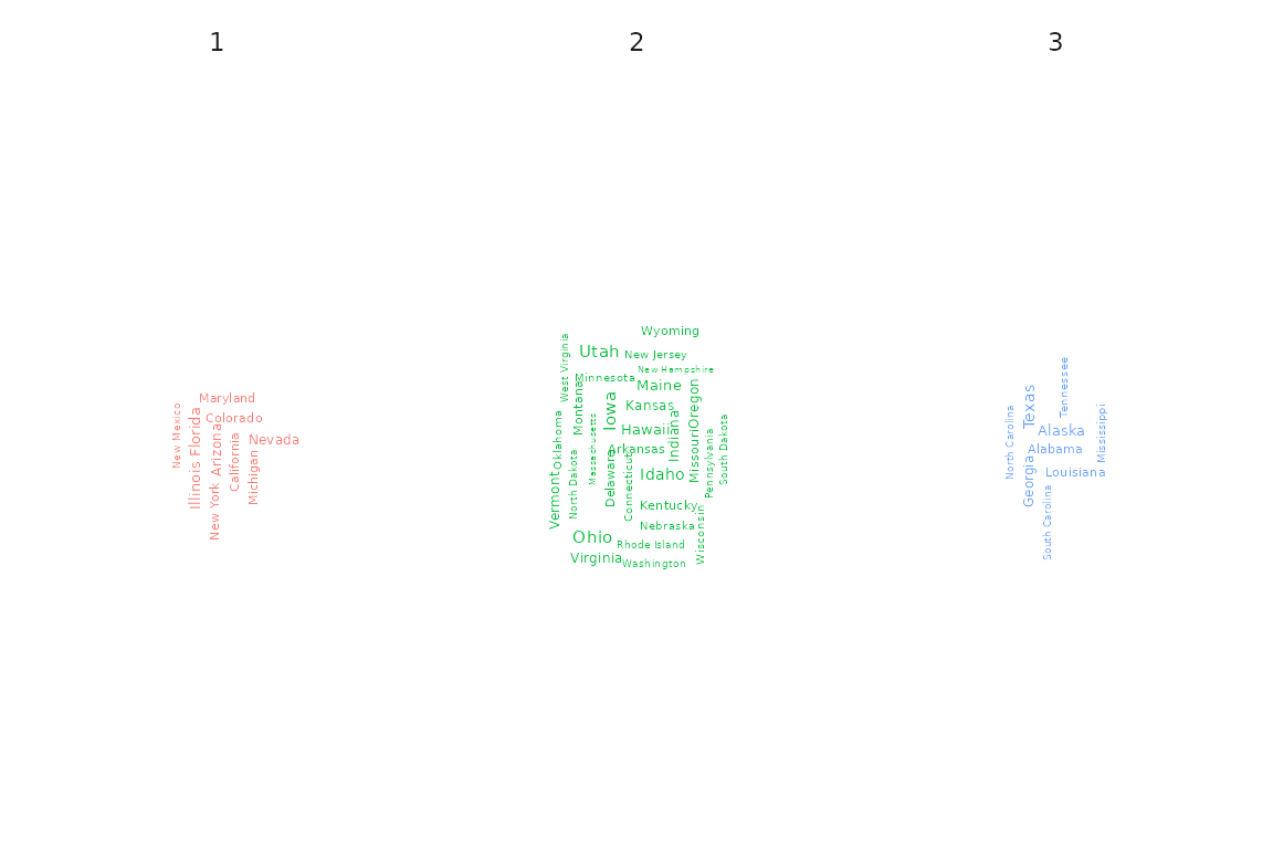
Plot of clustering results
# Enrich the USArrest dataset by area and state

USArrests_enriched <- USArrests %>%
  mutate(State = as.factor(rownames(USArrests)),
         Area  = as.factor(case_when(State %in% c("Washington", "Oregon",
                 "California", "Nevada", "Arizona", "Idaho", "Montana",
                 "Wyoming", "Colorado", "New Mexico", "Utah", "Hawaii",
                 "Alaska") ~ "West",
                 State %in% c("Texas", "Oklahoma", "Arkansas", "Louisiana",
                 "Mississippi", "Alabama", "Tennessee", "Kentucky", "Georgia",
                 "Florida", "South Carolina", "North Carolina", "Virginia",
                 "West Virginia") ~ "South",
                 State %in% c("Kansas", "Nebraska", "South Dakota",
                 "North Dakota", "Minnesota", "Missouri", "Iowa", "Illinois",
                 "Indiana", "Michigan", "Wisconsin", "Ohio") ~ "Midwest",
                 State %in% c("Maine", "New Hampshire", "New York",
                 "Massachusetts", "Rhode Island", "Vermont", "Pennsylvania",
                 "New Jersey", "Connecticut", "Delaware", "Maryland") ~
                   "Northeast")))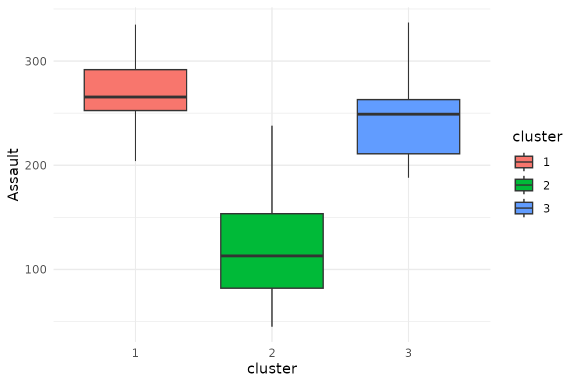
Scatterplot
plot(x = cc_fuzzy, data = USArrests_enriched, type = "scatterplot",
     x_var = "Murder", y_var = "Assault")
## `geom_smooth()` using formula = 'y ~ x'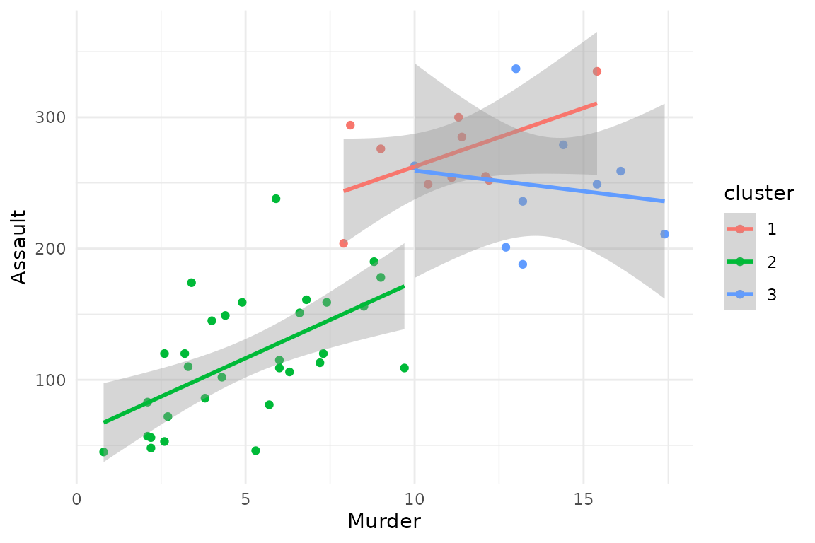
plot(x = cc_fuzzy, data = USArrests_enriched, type = "scatterplot",
     x_var = "Murder", y_var = "Assault",
     focus = TRUE)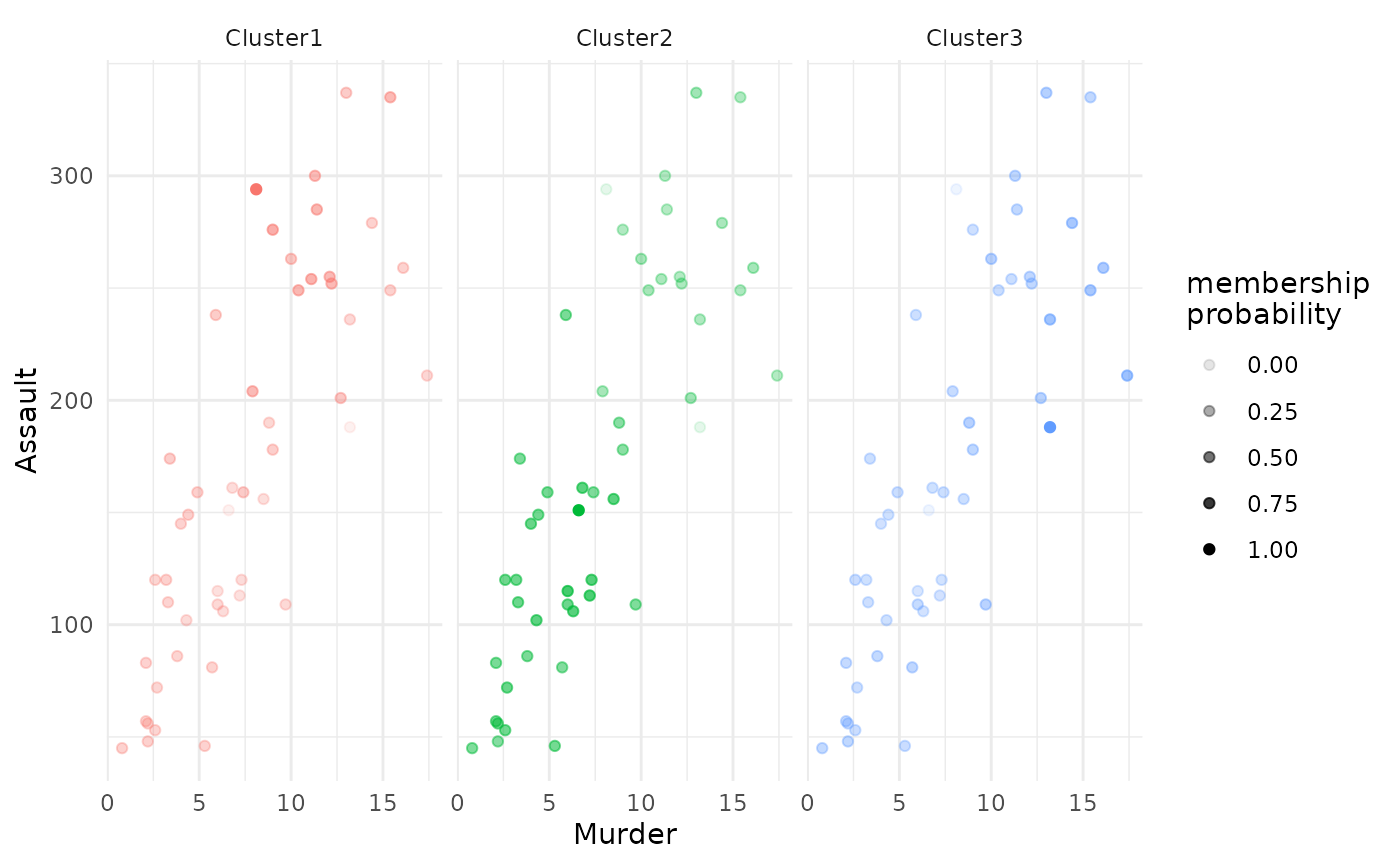
PCA
plot(x = cc_fuzzy, data = USArrests_enriched, type = "pca",
     group_by = "Area")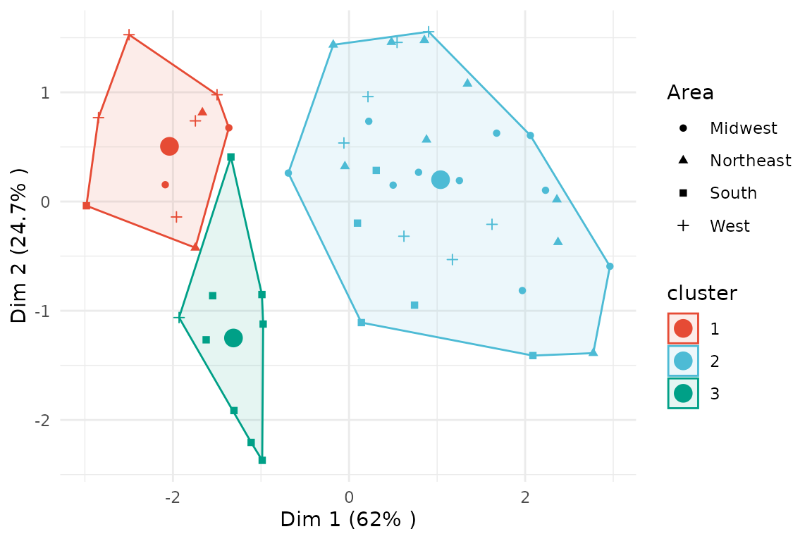
plot(x = cc_fuzzy, data = USArrests_enriched, type = "pca",
     focus = TRUE)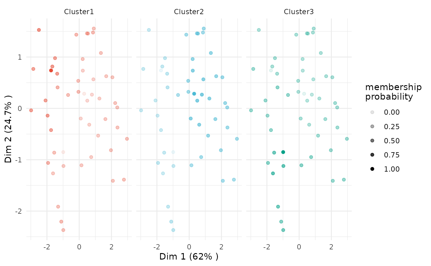
Silhouette
plot(x = cc_fuzzy, data = USArrests, type = "silhouette")## $plot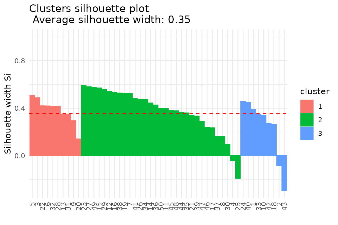
##
## $silhouette_table
##   Cluster Size Silhouette width
## 1       1   10        0.3802710
## 2       2   31        0.3786707
## 3       3    9        0.2383694
##
## $average_silhouette_width
## [1] 0.3537365