Visualization of clustering solution by variables
plot.fuzzyclara.RdFunction to provide graphical visualization of distribution
Usage
# S3 method for class 'fuzzyclara'
plot(
  x,
  data,
  type = NULL,
  variable = NULL,
  na.omit = FALSE,
  membership_threshold = 0,
  sample_percentage = 1,
  plot_membership_scores = FALSE,
  seed = 42,
  ...
)
Arguments
- x
An object of class "fuzzyclara"
- data
data.frame or matrix used for clustering
- type, variable
Type of plot. One of
c("barplot","boxplot","wordclouds",
"silhouette","pca","scatterplot", "parallel")
. Defaults to NULL, which either plots a barplot or a boxplot, depending on the class ofvariable.- na.omit
Should missing values be excluded for plotting? Defaults to FALSE.
- membership_threshold
Threshold for fuzzy clustering observations to be plotted. Must be a number between 0 and 1. Defaults to 0.
- sample_percentage
Percentage value that indicates which percentage of observations should randomly selected for representation the plot. Must be a number between 0 and 1. Defaults to 1.
- plot_membership_scores
Boolean value indicating whether the cluster membership scores for the observations should be indicated through line the transparency (TRUE) or not (FALSE). Defaults to FALSE.
- seed
random number seed (needed for
clara_wordcloudandclara_parallel)- ...
Further arguments for internal plot functions. For each type there is an internal plot function. See for example
?clara_pca.
Examples
# Prepare data for example (enrich the USArrest dataset by area and state)
library(dplyr)
#>
#> Attaching package: ‘dplyr’
#> The following objects are masked from ‘package:stats’:
#>
#> filter, lag
#> The following objects are masked from ‘package:base’:
#>
#> intersect, setdiff, setequal, union
USArrests_enriched <- USArrests %>%
mutate(State = as.factor(rownames(USArrests)),
Area = as.factor(case_when(State %in% c("Washington", "Oregon",
"California", "Nevada",
"Arizona", "Idaho", "Montana",
"Wyoming", "Colorado",
"New Mexico", "Utah", "Hawaii",
"Alaska") ~ "West",
State %in% c("Texas", "Oklahoma", "Arkansas",
"Louisiana", "Mississippi",
"Alabama", "Tennessee",
"Kentucky", "Georgia",
"Florida", "South Carolina",
"North Carolina", "Virginia",
"West Virginia") ~ "South",
State %in% c("Kansas", "Nebraska", "South Dakota",
"North Dakota", "Minnesota",
"Missouri", "Iowa", "Illinois",
"Indiana", "Michigan", "Wisconsin",
"Ohio") ~ "Midwest",
State %in% c("Maine", "New Hampshire", "New York",
"Massachusetts", "Rhode Island",
"Vermont", "Pennsylvania",
"New Jersey", "Connecticut",
"Delaware", "Maryland") ~
"Northeast")))
# Determine clusters that will be plotted
cc_hard <- fuzzyclara(data = USArrests,
clusters = 3,
metric = "euclidean",
samples = 1,
sample_size = NULL,
type = "hard",
seed = 3526,
verbose = 0)
cc_hard
#> Clustering results
#>
#> Medoids
#> [1] "New Mexico" "Oklahoma" "New Hampshire"
#>
#> Clustering
#> [1] 2 2 2 3 2 2 3 3 2 2 3 1 2 3 1 3 3 2 1 2 3 2 1 2 3 3 3 2 1 3 2 2 2 1 3 3 3 3
#> [39] 3 2 1 2 2 3 1 3 3 1 1 3
#>
#> Minimum average distance
#> [1] 1.180717
cc_fuzzy <- fuzzyclara(data = USArrests,
clusters = 3,
metric = "euclidean",
samples = 1,
sample_size = NULL,
type = "fuzzy",
m = 2,
seed = 3526,
verbose = 0)
cc_fuzzy
#> Clustering results
#>
#> Medoids
#> [1] "Oklahoma" "Arizona" "Tennessee"
#>
#> Clustering
#> [1] 3 3 1 2 1 1 2 2 1 3 2 2 1 2 2 2 2 3 2 1 2 1 2 3 2 2 2 1 2 2 1 1 3 2 2 2 2 2
#> [39] 2 3 2 3 3 2 2 2 2 2 2 2
#>
#> Minimum average weighted distance
#> [1] 1.94242
#>
#> Membership scores
#> Cluster1 Cluster2 Cluster3
#> Alabama 0.2040878 0.2391714 0.5567409
#> Alaska 0.3373655 0.2726496 0.3899849
#> Arizona 1.0000000 0.0000000 0.0000000
#> Arkansas 0.2075892 0.3966215 0.3957893
#> California 0.5401685 0.2248051 0.2350264
#> Colorado 0.4475538 0.2744007 0.2780455
#> Connecticut 0.2348136 0.5280016 0.2371848
#> Delaware 0.2906227 0.4701428 0.2392345
#> Florida 0.4443412 0.2316682 0.3239905
#> Georgia 0.2091524 0.2149396 0.5759081
#> Hawaii 0.2482766 0.4883161 0.2634073
#> Idaho 0.2209589 0.5129169 0.2661242
#> Illinois 0.4666698 0.2739684 0.2593617
#> Indiana 0.1344369 0.6694262 0.1961369
#> Iowa 0.2311216 0.4905457 0.2783327
#> Kansas 0.1310680 0.6999444 0.1689876
#> Kentucky 0.1917648 0.4401893 0.3680459
#> Louisiana 0.2560625 0.2412981 0.5026393
#> Maine 0.2396947 0.4695769 0.2907285
#> Maryland 0.4281216 0.2306369 0.3412416
#> Massachusetts 0.2682437 0.5043343 0.2274220
#> Michigan 0.4467571 0.2192029 0.3340400
#> Minnesota 0.2158369 0.5379562 0.2462069
#> Mississippi 0.2484292 0.2817416 0.4698292
#> Missouri 0.2669546 0.3898602 0.3431852
#> Montana 0.1922866 0.5233027 0.2844107
#> Nebraska 0.1814854 0.5935543 0.2249603
#> Nevada 0.4372644 0.2469118 0.3158237
#> New Hampshire 0.2351771 0.4821286 0.2826942
#> New Jersey 0.3025875 0.4474846 0.2499279
#> New Mexico 0.4736616 0.2098122 0.3165261
#> New York 0.4959333 0.2489337 0.2551329
#> North Carolina 0.2984813 0.2995500 0.4019686
#> North Dakota 0.2525175 0.4409055 0.3065770
#> Ohio 0.1722044 0.6264071 0.2013885
#> Oklahoma 0.0000000 1.0000000 0.0000000
#> Oregon 0.2597840 0.4842455 0.2559705
#> Pennsylvania 0.1733916 0.6187011 0.2079073
#> Rhode Island 0.2938264 0.4548769 0.2512968
#> South Carolina 0.2521289 0.2569116 0.4909595
#> South Dakota 0.2294820 0.4627901 0.3077278
#> Tennessee 0.0000000 0.0000000 1.0000000
#> Texas 0.3315450 0.2977964 0.3706587
#> Utah 0.2550652 0.5204090 0.2245258
#> Vermont 0.2537642 0.4173744 0.3288614
#> Virginia 0.1470128 0.6016305 0.2513568
#> Washington 0.2420740 0.5403595 0.2175666
#> West Virginia 0.2356115 0.4301945 0.3341939
#> Wisconsin 0.2298126 0.5057011 0.2644864
#> Wyoming 0.1652925 0.6041126 0.2305949
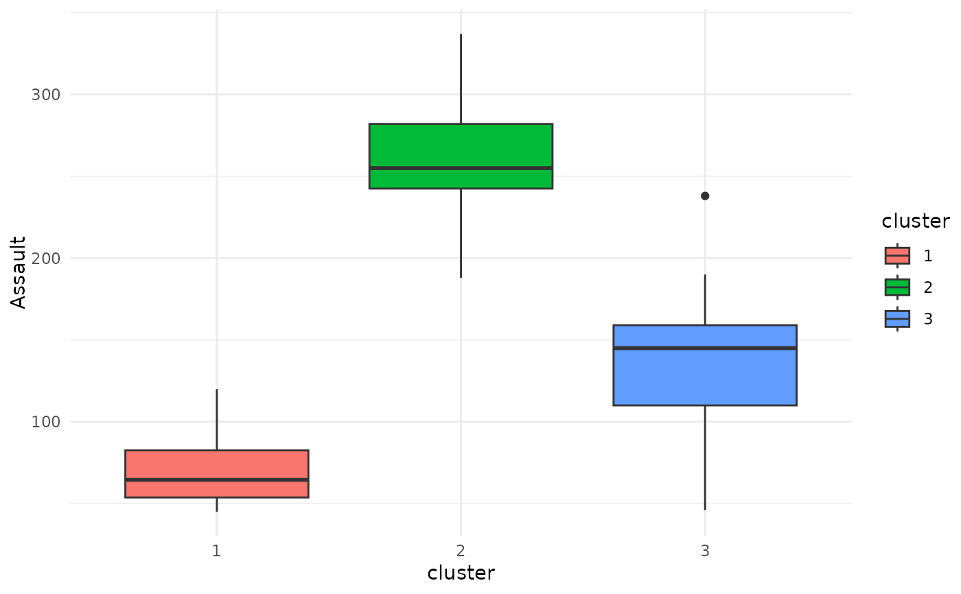
# Boxplot
plot(x = cc_hard, data = USArrests_enriched, variable = "Assault")
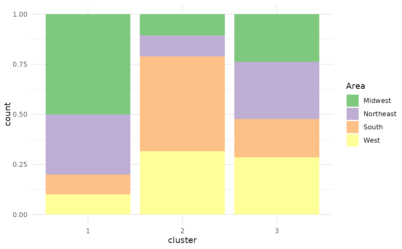
 # Barplot
plot(x = cc_hard, data = USArrests_enriched, variable = "Area")
# Barplot
plot(x = cc_hard, data = USArrests_enriched, variable = "Area")
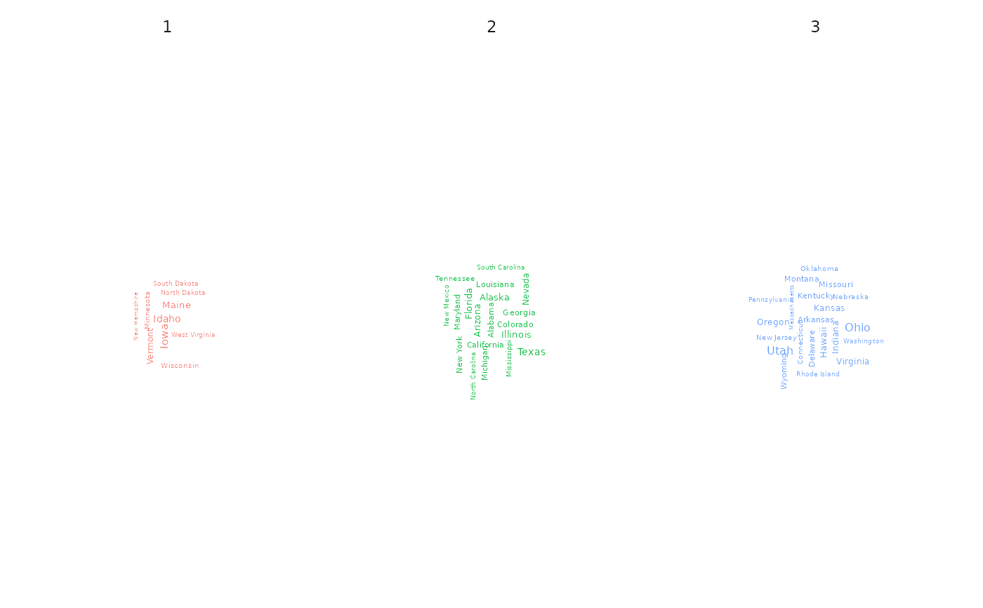
 # Wordcloud
plot(x = cc_hard, data = USArrests_enriched, variable = "State",
type = "wordclouds", seed = 123)
# Wordcloud
plot(x = cc_hard, data = USArrests_enriched, variable = "State",
type = "wordclouds", seed = 123)
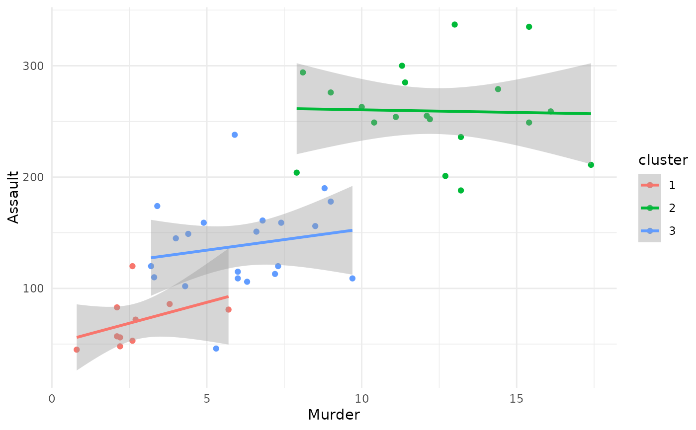
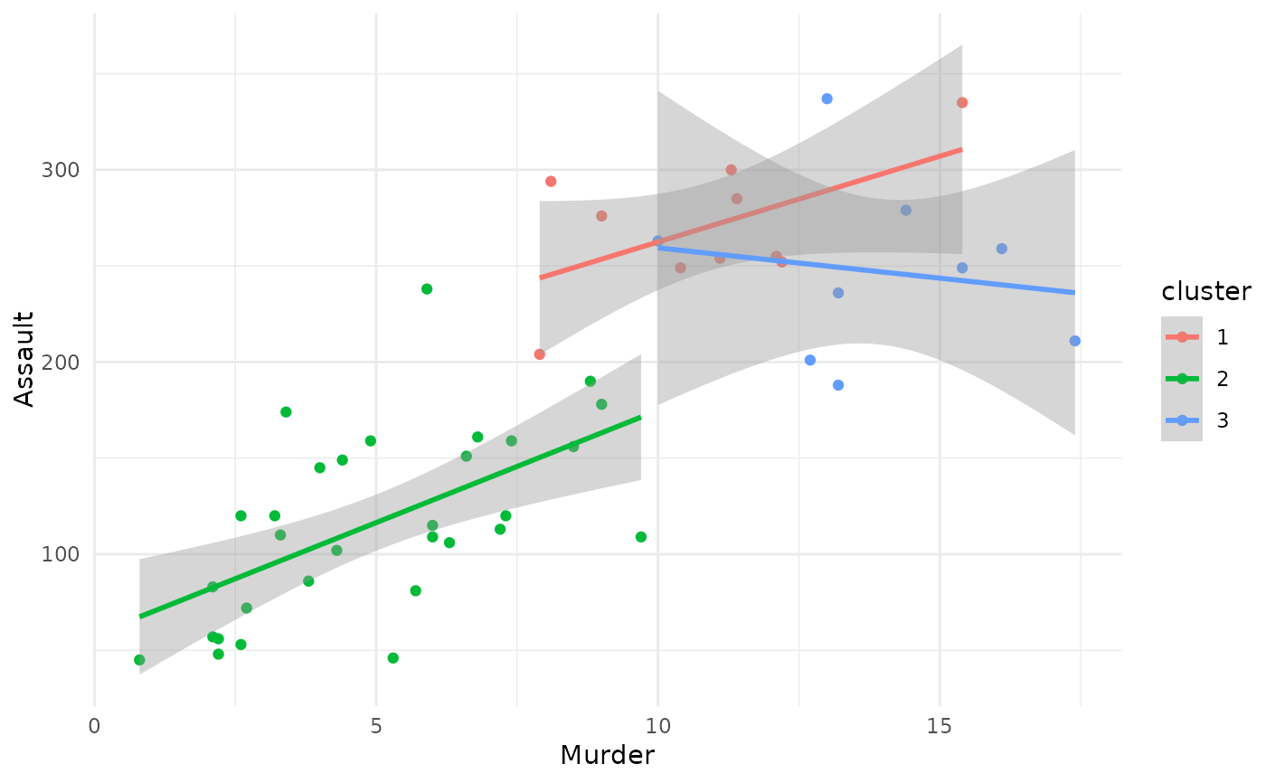
 # Scatterplot
plot(x = cc_hard, data = USArrests_enriched, type = "scatterplot",
x_var = "Murder", y_var = "Assault")
#> `geom_smooth()` using formula = 'y ~ x'
# Scatterplot
plot(x = cc_hard, data = USArrests_enriched, type = "scatterplot",
x_var = "Murder", y_var = "Assault")
#> `geom_smooth()` using formula = 'y ~ x'
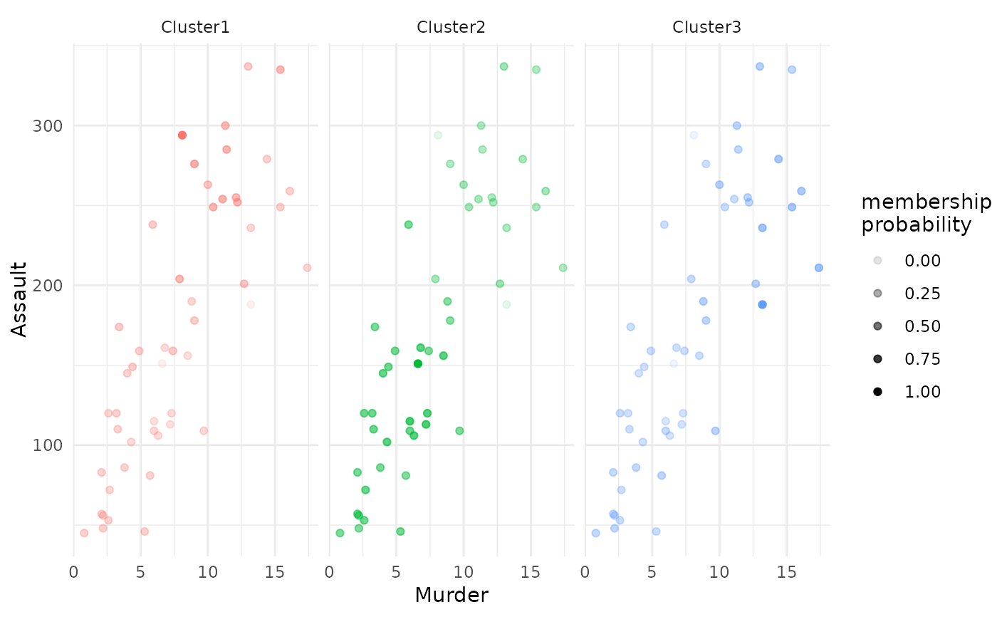
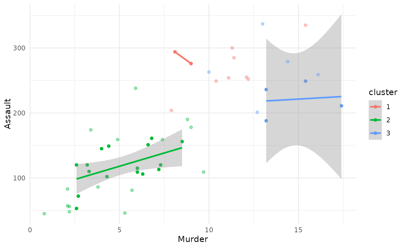
 # Plot membership probability for fuzzy clustering
plot(x = cc_fuzzy, data = USArrests_enriched, type = "scatterplot",
x_var = "Murder", y_var = "Assault",
focus = TRUE)
# Plot membership probability for fuzzy clustering
plot(x = cc_fuzzy, data = USArrests_enriched, type = "scatterplot",
x_var = "Murder", y_var = "Assault",
focus = TRUE)
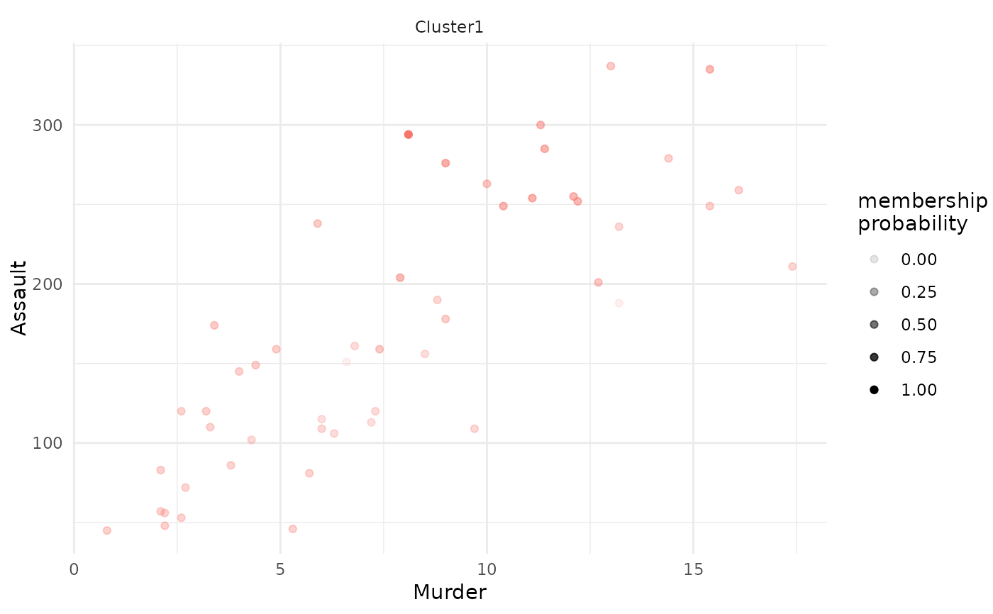
 # Plot membership probability for fuzzy clustering (one cluster only)
plot(x = cc_fuzzy, data = USArrests_enriched, type = "scatterplot",
x_var = "Murder", y_var = "Assault",
focus = TRUE, focus_clusters = c(1))
# Plot membership probability for fuzzy clustering (one cluster only)
plot(x = cc_fuzzy, data = USArrests_enriched, type = "scatterplot",
x_var = "Murder", y_var = "Assault",
focus = TRUE, focus_clusters = c(1))
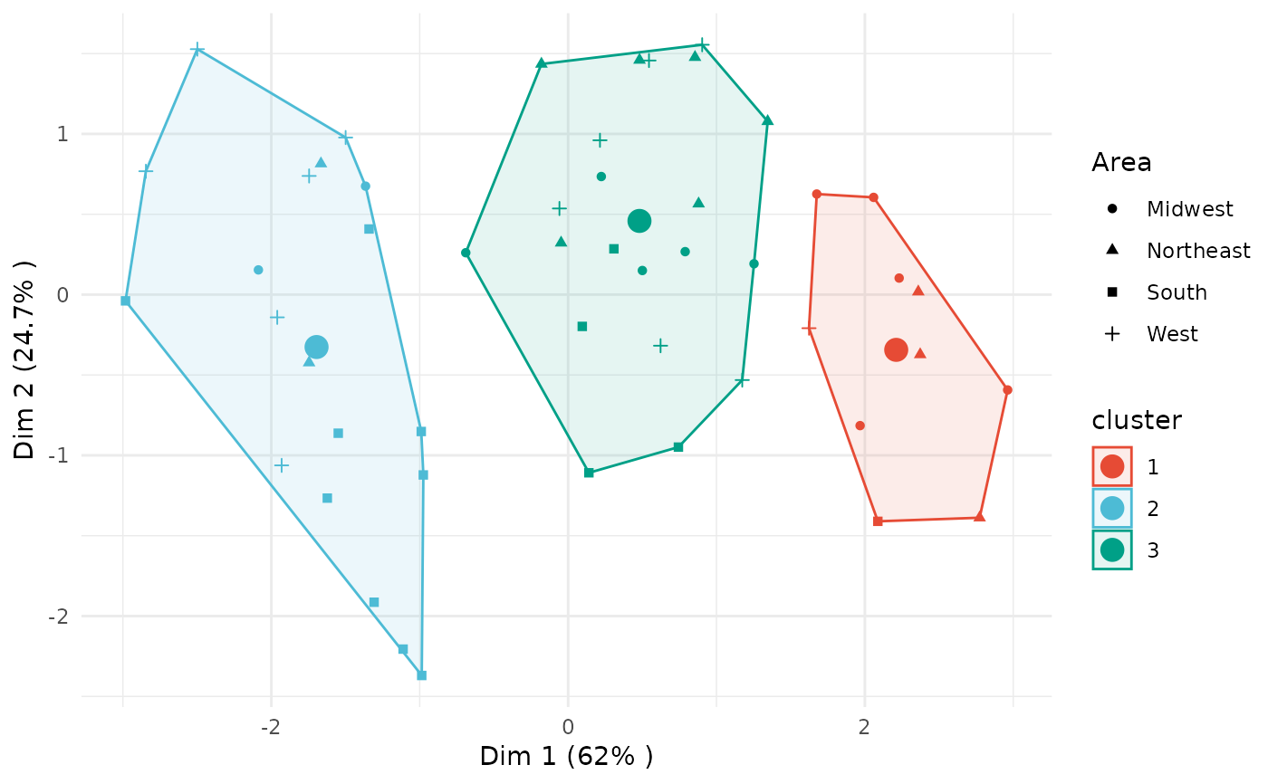
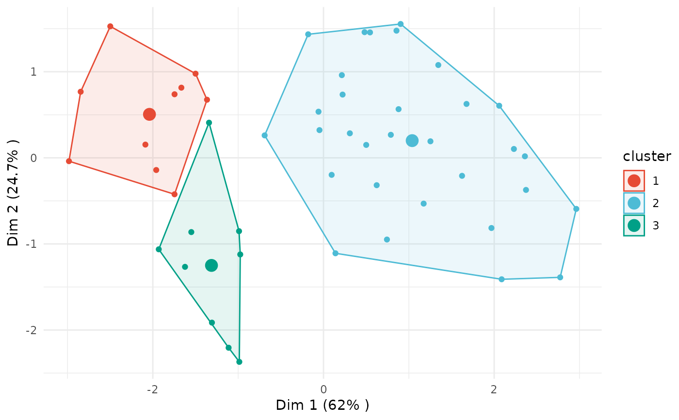
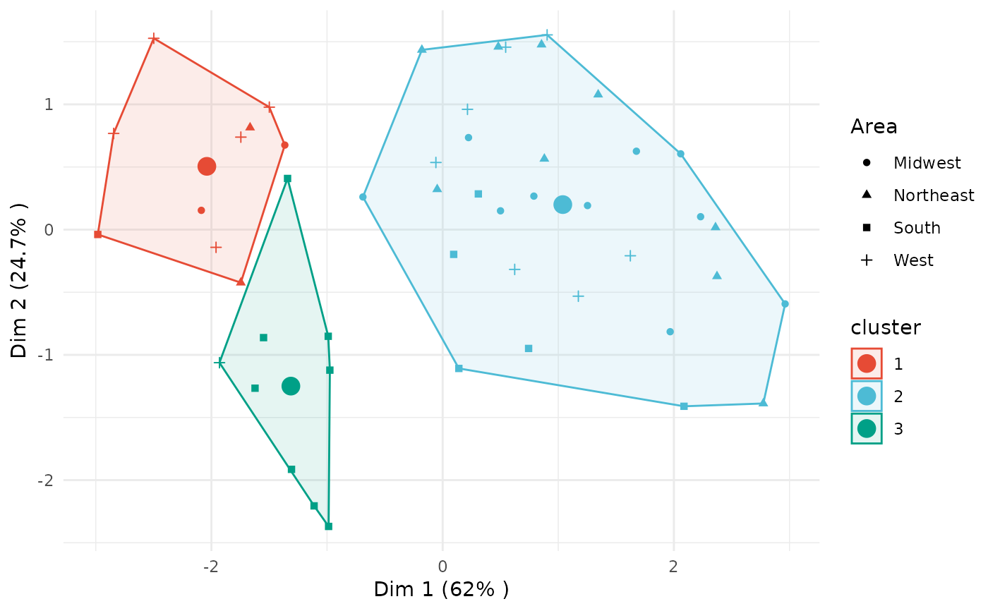
 # PCA
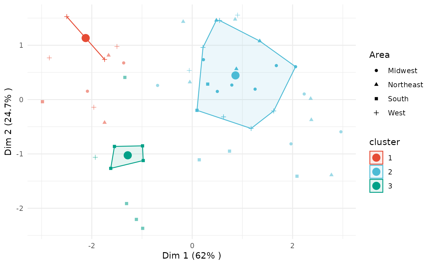
plot(x = cc_hard, data = USArrests_enriched, type = "pca",
group_by = "Area")
# PCA
plot(x = cc_hard, data = USArrests_enriched, type = "pca",
group_by = "Area")
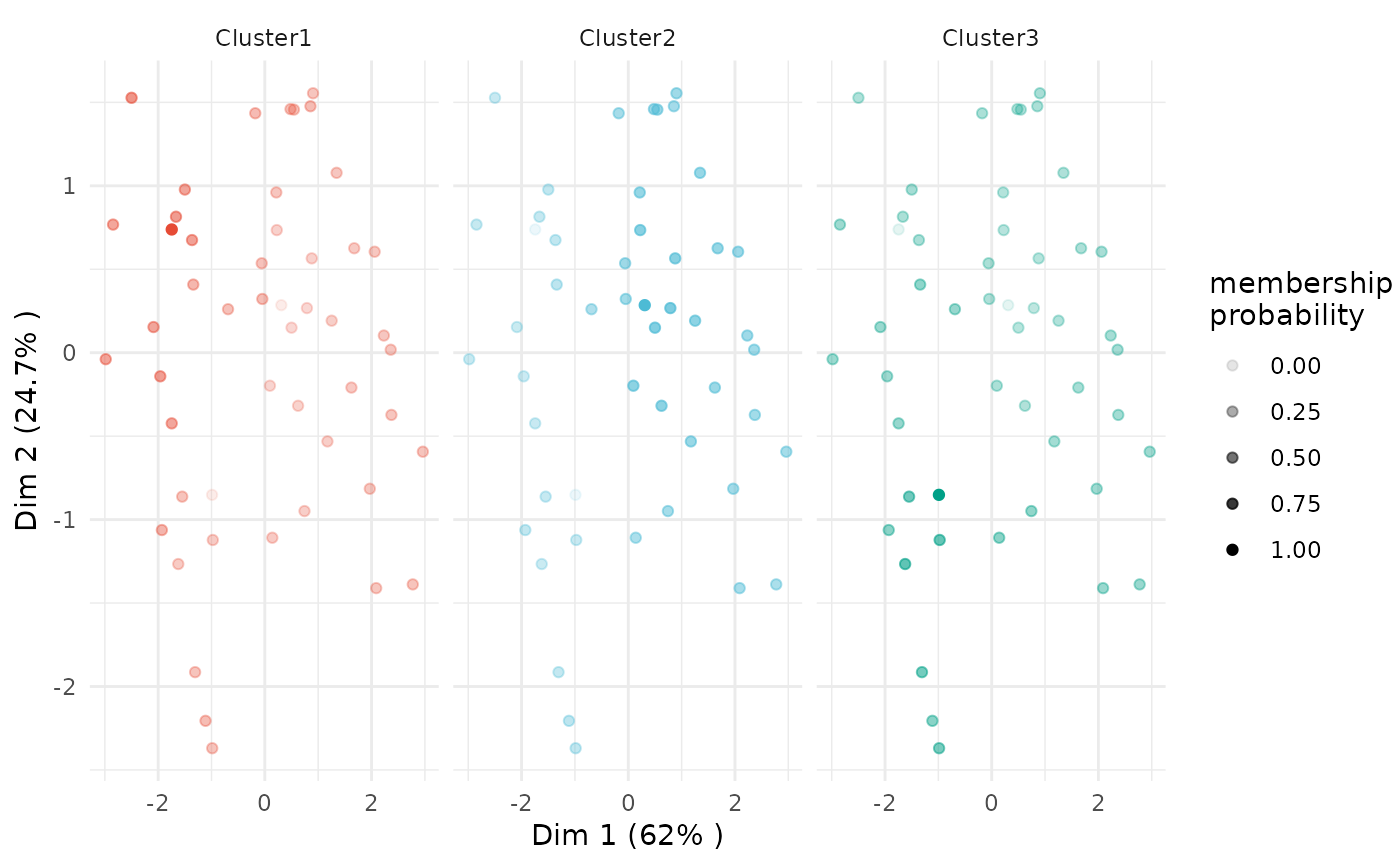
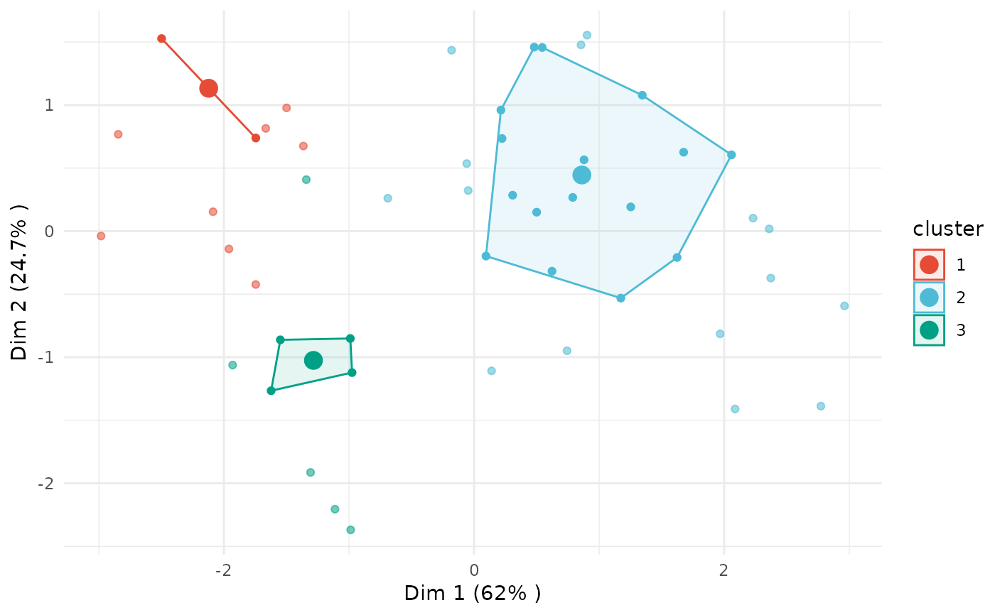
 # Plot membership probability for one or more clusters following a PCA
plot(x = cc_fuzzy, data = USArrests_enriched, type = "pca",
focus = TRUE)
# Plot membership probability for one or more clusters following a PCA
plot(x = cc_fuzzy, data = USArrests_enriched, type = "pca",
focus = TRUE)
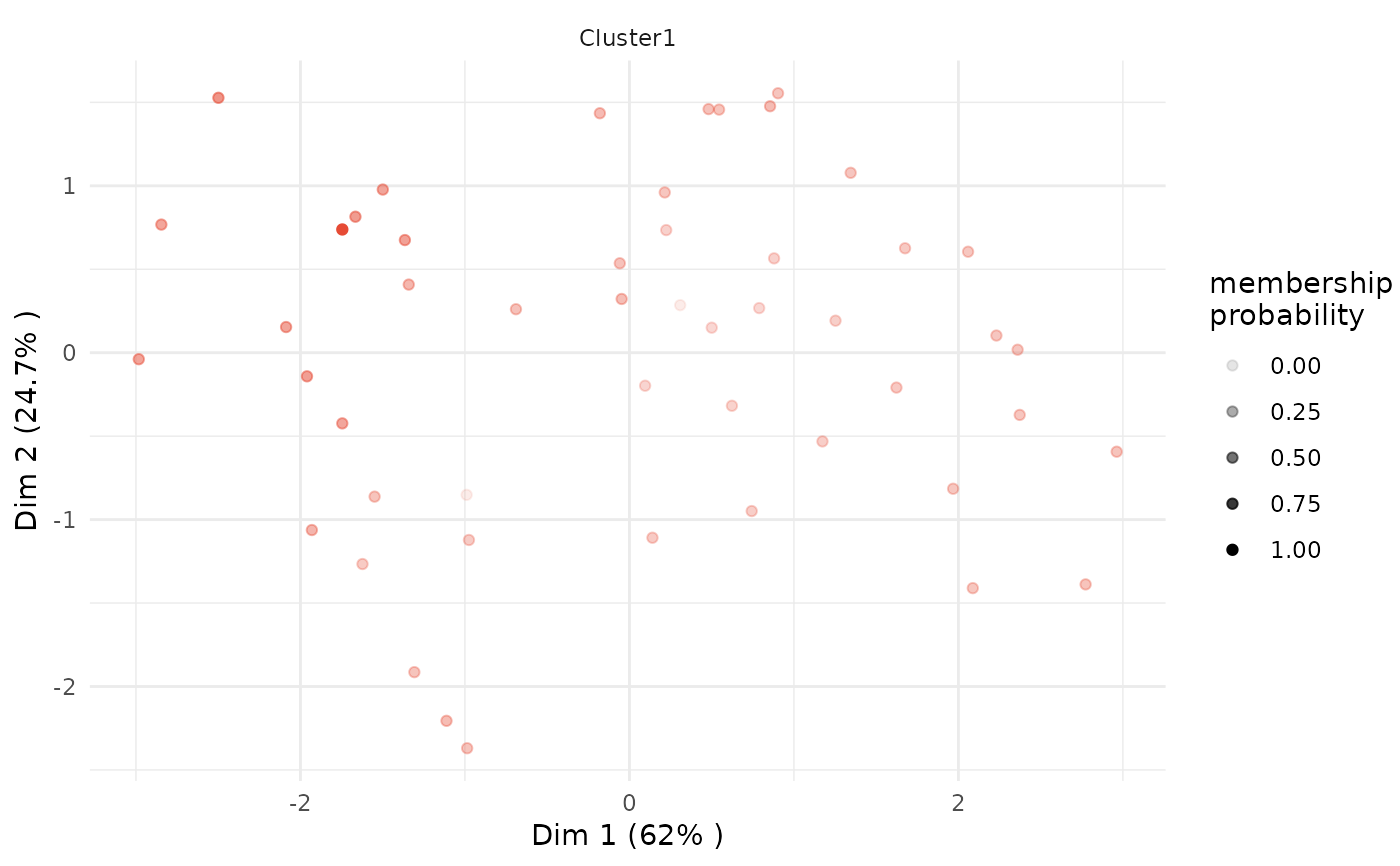
 plot(x = cc_fuzzy, data = USArrests_enriched, type = "pca",
focus = TRUE, focus_clusters = c(1))
plot(x = cc_fuzzy, data = USArrests_enriched, type = "pca",
focus = TRUE, focus_clusters = c(1))
 # Silhouette plot
plot(x = cc_hard, data = USArrests, type = "silhouette")
#> $plot
# Silhouette plot
plot(x = cc_hard, data = USArrests, type = "silhouette")
#> $plot
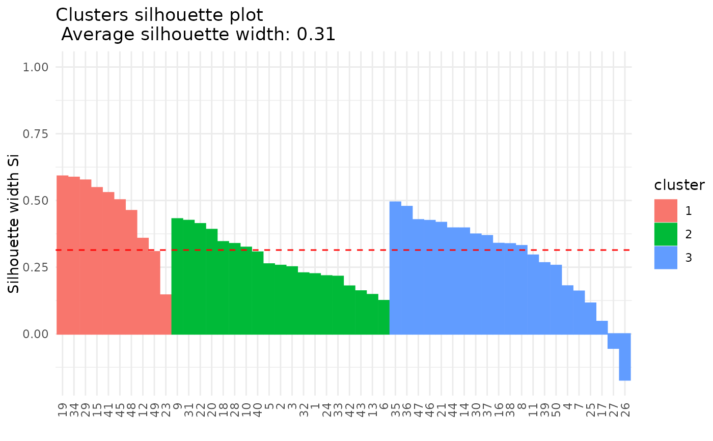 #>
#> $silhouette_table
#> Cluster Size Silhouette width
#> 1 1 10 0.4604416
#> 2 2 19 0.2757843
#> 3 3 21 0.2797126
#>
#> $average_silhouette_width
#> [1] 0.3143656
#>
# Plot clusters for fuzzy clustering (using threshold for membership scores)
plot(x = cc_fuzzy, data = USArrests_enriched, type = "pca",
variable = "Assault", membership_threshold = 0)
#>
#> $silhouette_table
#> Cluster Size Silhouette width
#> 1 1 10 0.4604416
#> 2 2 19 0.2757843
#> 3 3 21 0.2797126
#>
#> $average_silhouette_width
#> [1] 0.3143656
#>
# Plot clusters for fuzzy clustering (using threshold for membership scores)
plot(x = cc_fuzzy, data = USArrests_enriched, type = "pca",
variable = "Assault", membership_threshold = 0)
 plot(x = cc_fuzzy, data = USArrests_enriched, type = "pca",
variable = "Assault", membership_threshold = 0.5)
plot(x = cc_fuzzy, data = USArrests_enriched, type = "pca",
variable = "Assault", membership_threshold = 0.5)
 plot(x = cc_fuzzy, data = USArrests_enriched, type = "scatterplot",
x_var = "Murder", y_var = "Assault", membership_threshold = 0)
#> `geom_smooth()` using formula = 'y ~ x'
plot(x = cc_fuzzy, data = USArrests_enriched, type = "scatterplot",
x_var = "Murder", y_var = "Assault", membership_threshold = 0)
#> `geom_smooth()` using formula = 'y ~ x'
 plot(x = cc_fuzzy, data = USArrests_enriched, type = "scatterplot",
x_var = "Murder", y_var = "Assault", membership_threshold = 0.5)
#> `geom_smooth()` using formula = 'y ~ x'
#> Warning: NaNs produced
#> Warning: no non-missing arguments to max; returning -Inf
plot(x = cc_fuzzy, data = USArrests_enriched, type = "scatterplot",
x_var = "Murder", y_var = "Assault", membership_threshold = 0.5)
#> `geom_smooth()` using formula = 'y ~ x'
#> Warning: NaNs produced
#> Warning: no non-missing arguments to max; returning -Inf
 plot(x = cc_fuzzy, data = USArrests_enriched, type = "scatterplot",
x_var = "Murder", y_var = "Assault", membership_threshold = 0.5,
plot_all_fuzzy = TRUE)
#> `geom_smooth()` using formula = 'y ~ x'
#> Warning: NaNs produced
#> Warning: no non-missing arguments to max; returning -Inf
plot(x = cc_fuzzy, data = USArrests_enriched, type = "scatterplot",
x_var = "Murder", y_var = "Assault", membership_threshold = 0.5,
plot_all_fuzzy = TRUE)
#> `geom_smooth()` using formula = 'y ~ x'
#> Warning: NaNs produced
#> Warning: no non-missing arguments to max; returning -Inf
 plot(x = cc_fuzzy, data = USArrests_enriched, type = "pca",
group_by = "Area", membership_threshold = 0)
plot(x = cc_fuzzy, data = USArrests_enriched, type = "pca",
group_by = "Area", membership_threshold = 0)
 plot(x = cc_fuzzy, data = USArrests_enriched, type = "pca",
group_by = "Area", membership_threshold = 0.5)
plot(x = cc_fuzzy, data = USArrests_enriched, type = "pca",
group_by = "Area", membership_threshold = 0.5)
 plot(x = cc_fuzzy, data = USArrests_enriched, type = "pca",
group_by = "Area", membership_threshold = 0.5, plot_all_fuzzy = TRUE)
plot(x = cc_fuzzy, data = USArrests_enriched, type = "pca",
group_by = "Area", membership_threshold = 0.5, plot_all_fuzzy = TRUE)
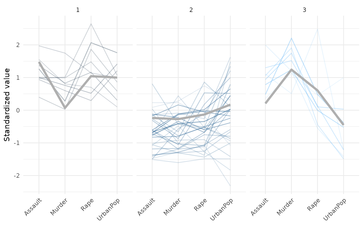
 # Parallel Plot
plot(x = cc_fuzzy, data = USArrests_enriched,
type = "parallel", sample_percentage = 1, plot_membership_scores = TRUE)
# Parallel Plot
plot(x = cc_fuzzy, data = USArrests_enriched,
type = "parallel", sample_percentage = 1, plot_membership_scores = TRUE)