Joint plot to compare the marginal APC effects of multiple models

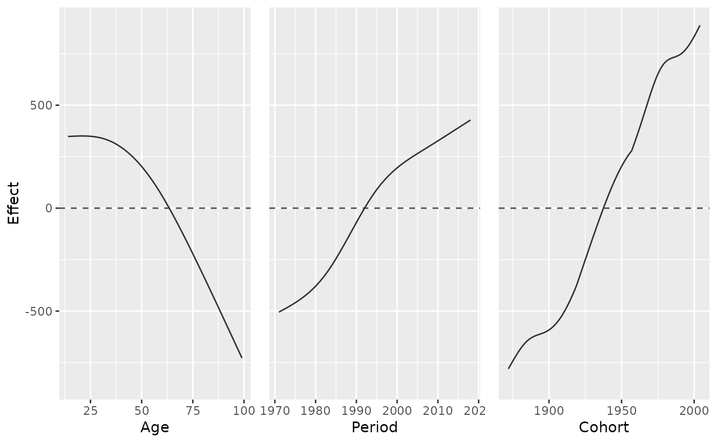
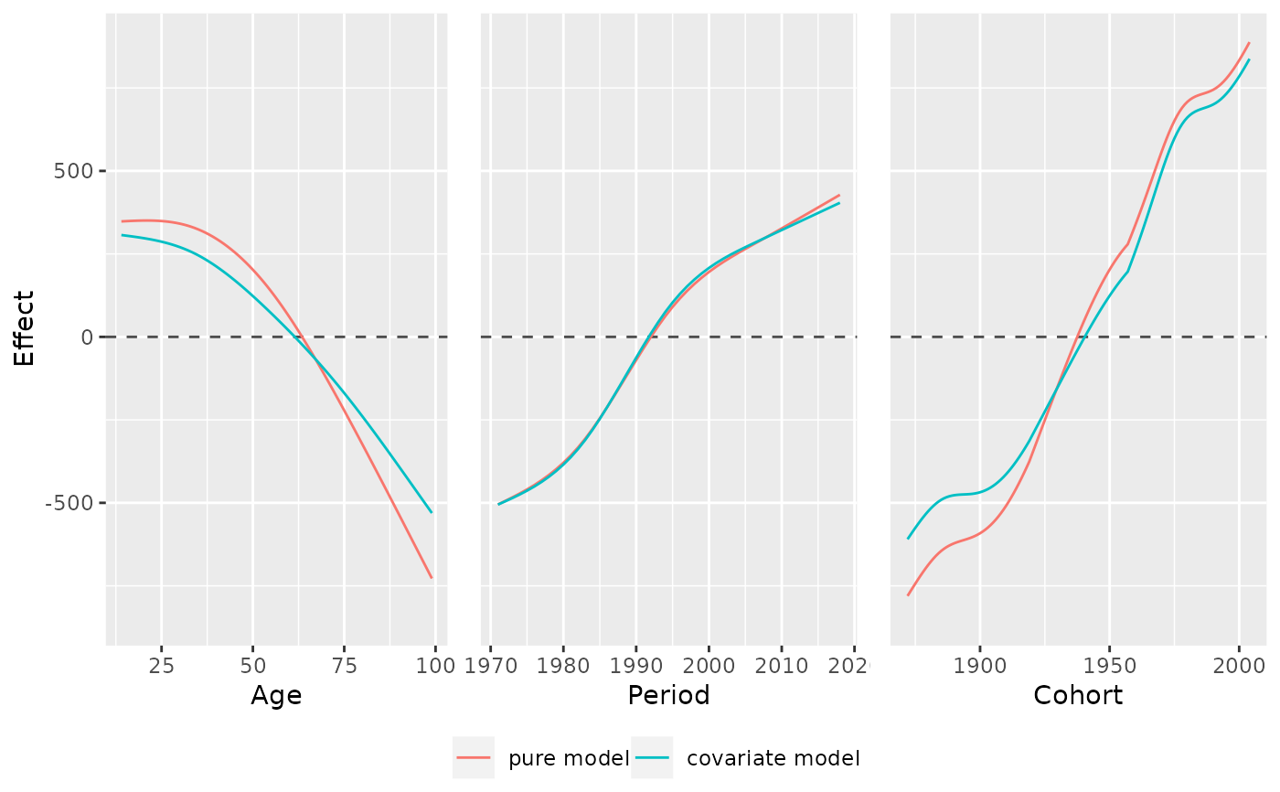
This function creates a joint plot of the marginal APC effects of multiple estimated models. It creates a plot with one pane per age, period and cohort effect, each containing one lines for each estimated model.

Usage

plot_jointMarginalAPCeffects(
  model_list,
  dat,
  vlines_list = NULL,
  ylab = NULL,
  ylim = NULL,
  plot_CI = FALSE
)

Arguments

model_list

A list of regression models estimated with gam or bam. If the list is named, the names are used as labels. Can also be a single model object instead of a list.

dat

Dataset with columns period and age. If y_var is specified, the dataset must contain the respective column. If model is specified, the dataset must have been used for model estimation with gam or bam.

vlines_list

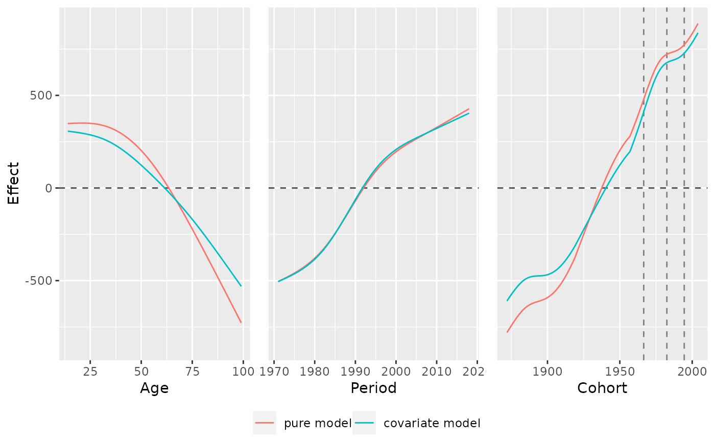
Optional list that can be used to highlight the borders of specific age groups, time intervals or cohorts. Each element must be a numeric vector of values on the x-axis where vertical lines should be drawn. The list can maximally have three elements and must have names out of c("age","period","cohort".

ylab, ylim

Optional ggplot2 styling arguments.

plot_CI

Indicator if 95% confidence intervals should be plotted. Defaults to FALSE.

Value

Plot grid created with ggarrange.

Details

If the model was estimated with a log or logit link, the function automatically performs an exponential transformation of the effect.

Since the plot output created by the function is no ggplot2 object, but an object created with ggpubr::ggarrange, the overall theme of the plot cannot be changed by adding the theme in the form of 'plot_jointMarginalAPCeffects(...) + theme_minimal(...)'. Instead, you can call theme_set(theme_minimal(...)) as an individual call before calling plot_jointMarginalAPCeffects(...). The latter function will then use this global plotting theme.

Author

Alexander Bauer alexander.bauer@stat.uni-muenchen.de, Maximilian Weigert maximilian.weigert@stat.uni-muenchen.de

Examples

library(APCtools)
library(mgcv)

data(travel)

# plot marginal effects of one model
model_pure <- gam(mainTrip_distance ~ te(age, period), data = travel)
plot_jointMarginalAPCeffects(model_pure, dat = travel)


# plot marginal effects of multiple models
model_cov  <- gam(mainTrip_distance ~ te(age, period) + s(household_income),
                  data = travel)
model_list <- list("pure model"      = model_pure,
                   "covariate model" = model_cov)
plot_jointMarginalAPCeffects(model_list, dat = travel)


# mark specific cohorts
plot_jointMarginalAPCeffects(model_list, dat = travel,
                             vlines_list = list("cohort" = c(1966.5,1982.5,1994.5)))